On Vineyards, Harmony, and Mathematics

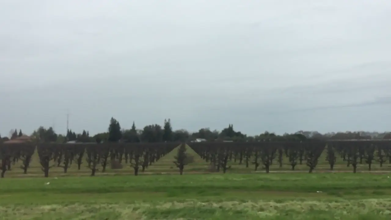
Whether it was my father’s profession as a Winemaker, or the frequency of my time spent in the back seat of the car as a kid on long drives through the Central Valley of California, watching vineyards pass by on endless pastoral back-roads was one of the most distinct memories of my youth. It was easy to find myself lost in the mesmerizing patterns of gaps between posts as they flew by. A beautiful and curious event, no doubt, but one that I didn’t ascribe much more meaning to than the mountains far off in the distance or the winding aqueducts that provided sustenance for so many crops. I never could have anticipated that these seemingly prosaic forms emerging from the vines were a tangible window into a prolific structure at the foundation of music theory, quantum mechanics, self-organized criticality, number theory, and dynamical systems. In this post I hope to share the intimate connection with music, and later share additional relationships that are related in surprising ways.

Caveats

For the majority of my life, I have enjoyed playing the guitar. I was lucky enough to receive lessons when I was in middle school and was able to practice to a point where I could feel comfortable playing a few songs. I never have thought of myself as a musician, and a large part of that has been my struggle with the theory. Unlike my math classes, music theory classes required much memorization and there were many questions I had that went unanswered. I admire others’ ability to memorize the usage of tools and apply them, but I lack that gift and only feel comfortable in fields where I can understand where the tools came from and why they work. Still, unlike other classes where the lines drawn around meaning were more subjective, music theory always seemed to tease at a deeper meaning that was derivable from first principles, yet whenever I asked about the “how” the answer was invariably related to another piece of memorization or an appeal to tradition.

While I fully accept that much of music theory and its application is rooted in tradition and rich in global culture, I recently found satisfying answers to my questions that are far more axiomatic. Also, I’ll add that my understanding of music theory is still developing and what I share here only touches on fundamentals, and the foundations that produce them. Still, if you are someone who is well versed in music theory I hope that this article will provide some useful intuition around the origins of music theory.

Notes as Tones

It would come as no surprise that music consists of periodic vibrations in the air. When I was little, I remember the first time I learned about speakers, and my subsequent confusion as to how such a device could even function. One note can be described as a pure pitch, oscillating some given amount of times per second (measured in Hertz or Hz). How could one physical object play two notes, or even thousands of them at the same time? In the same vein, how could one object moving in time produce the sound of someone singing and a guitar playing simultaneously?

It turns out that any sound can be decomposed into an infinite sum of pure pitches in a process known as Fourier decomposition. Any signal can be equivalently described by its frequency spectrum, and in many cases this provides an extremely useful context for analyzing things like sound and music that would be impossible without it. In the case of a speaker vibrating, it is the ability for these individual pitches to sum together in Superposition that allows one object to produce so many sounds simultaneously.

While it won’t be very useful at the moment to dive deeper into topics like Fourier Analysis, I recommend reading about the subject in the future if you haven’t had the chance. It is one of the most beautiful pieces of math I have ever encountered. For now, I just wanted to present the view of notes as waves in time. As you might guess, another view of sound involves waves in space.

Wave-Like Phenomena

A staggering amount of physical systems exhibit wave-like behavior. To adequately articulate what that means, I would have to touch on the ubiquitous wave equation, which has some nuance and prerequisite knowledge of differential equations. It is sufficient now to know that the motion of a vibrating string, or air oscillating in a horn is described by the wave equation. A consequence of these kinds of system is that they have many stable configurations of motion called modes (or harmonics). Speaking of a string instrument, when you pluck an individual string there will be a fundamental harmonic determined by the tension, length, and mass of the string. Above that fundamental in pitch will be a second harmonic at double the initial frequency. Above that will be another with three times the initial frequency, then four, and so on. This is because the string is free to move in any way that is permitted by its constraints (the beginning and end of the string must remain still). As the peaks and valleys of the vibrations must be all of the same size (otherwise tension would make them so) a string will have harmonics at integer multiples of the fundamental. If you follow these two constraints, this integer progression of frequency is the only possible outcome of motion.

In music, this is called the harmonic series. When we speak of notes on instruments, we refer to their fundamental. The note “A” is defined to be 440Hz, but the amplitude of harmonics produced by different instruments playing the same note will differ greatly. In some circumstances (as is the case with horns) only some of the harmonics will be present. Horns are different from strings in that one end of the system is open to the air, and the other closed. Such a system produces odd harmonics (1, 3, 5, and so on) as, unlike the string, one end is allowed to move freely.

Still, the harmonic series is general enough to apply to the theory of most instruments, and it will help us answer one of my most fundamental questions about music theory: what makes a given interval sound good?

Intervals

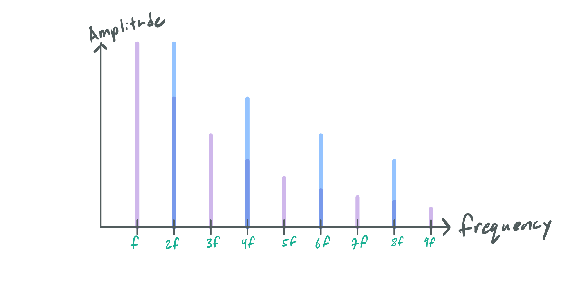
Musical intervals lie at the heart of music theory. An interval is simply the ratio of a note with respect to another (called the root). For instance, the octave interval is a doubling (meaning a ratio of \(2:1\)). One curious property of intervals, is that some of them sound pleasant, and some are so dissonant that they evoke religious allusion to the devil. Certain intervals seem to be more recognizable than others in music, and the quality of two notes sounding like each other (or good with another, which is closely related as we will soon see) is called consonance (the opposite of dissonance). Starting with the most simple interval (unity, or \(1:1\)), it makes sense that two notes of the same pitch will sound equivalent. Less intuitive is the octave: why does a doubling in frequency yield a note that sounds the same as the root? To answer that question, we can apply our knowledge of the Harmonic Series. Here is what a note might look like if we broke it down into its harmonics:

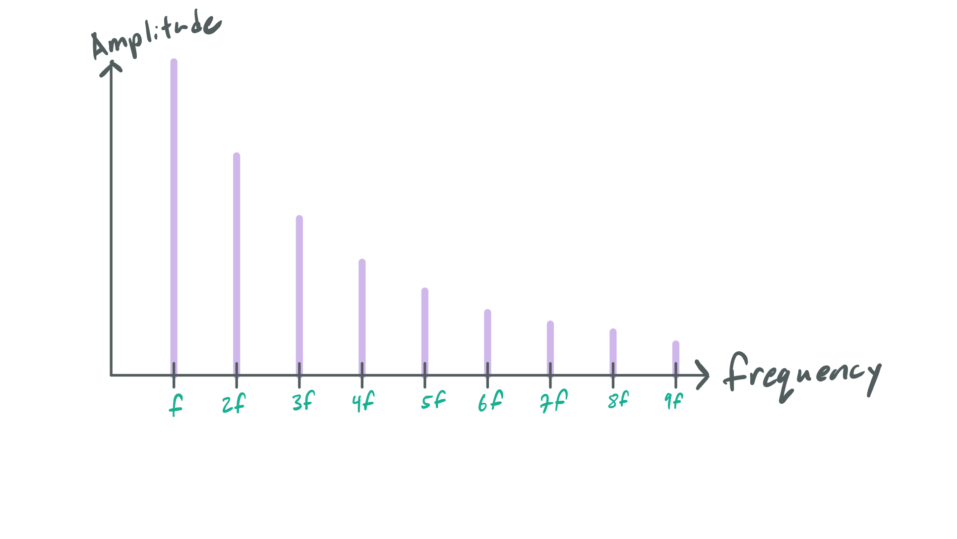
Here \(f\) stands for the fundamental pitch or frequency, and each harmonic is an integer multiple above it. The amplitude of the harmonics decrease as the order increases. The timbre of an instrument can be partly attributed to this distribution, but for now we are only concerned with the periodic structure of the harmonics in the frequency domain. Keeping \(f\) constant, here is the spectrum of a note one octave above the root (\(2:1\) or double the frequency):

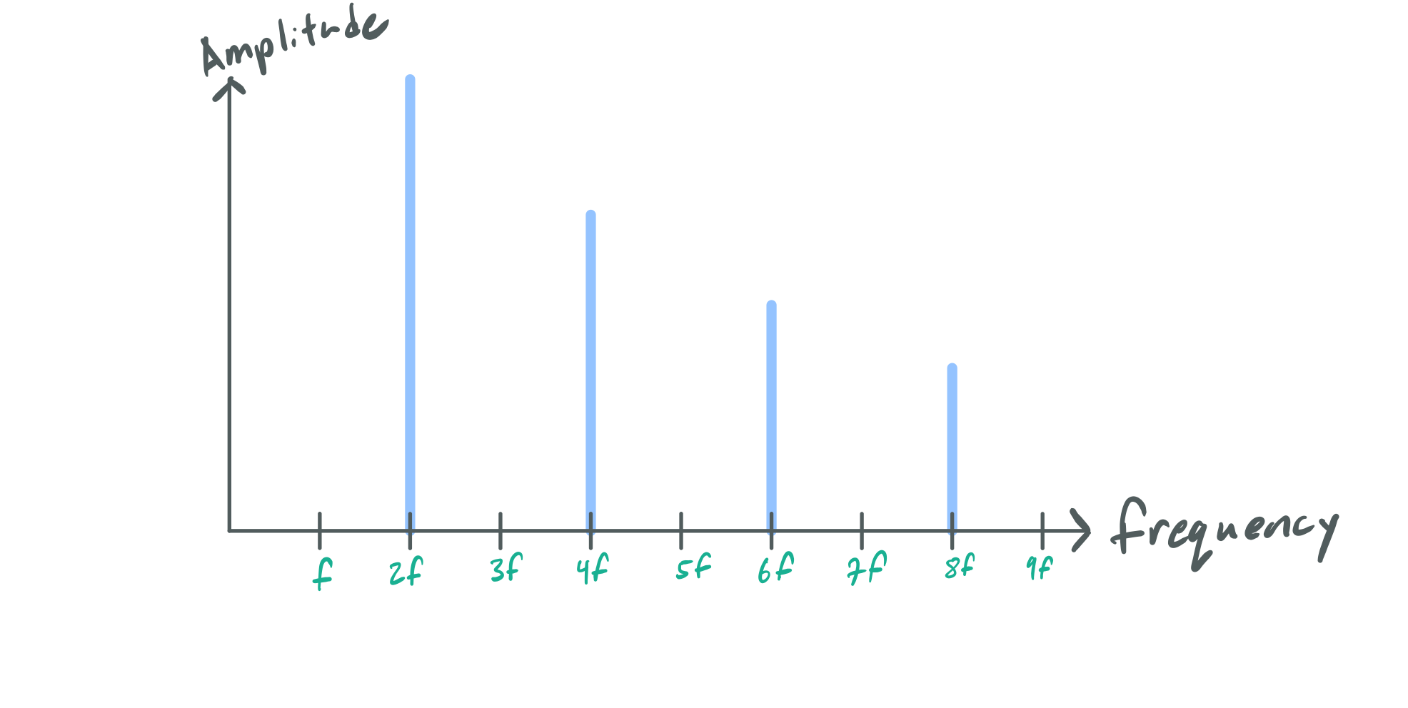
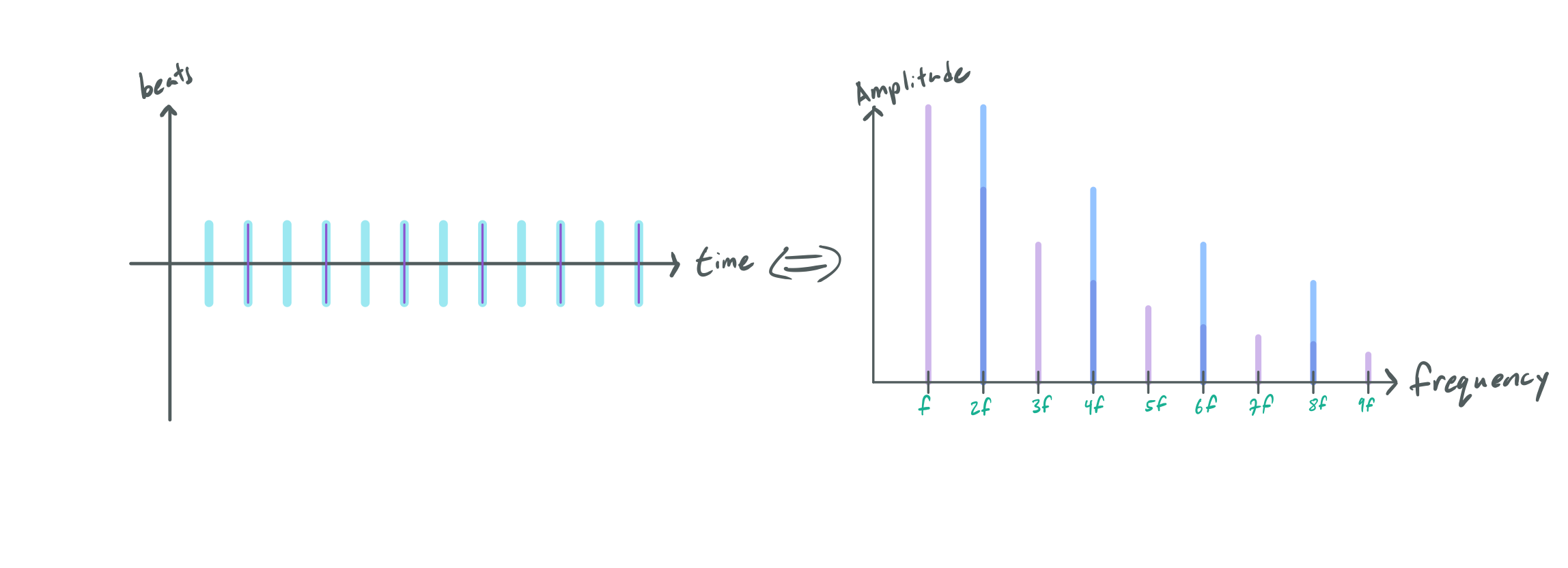
This is the same envelope as before, but stretched out by a factor of two. Likewise, each harmonic is now scaled by a factor of two as well. To see why these two notes sound identical, we can overlay the two distributions to compare them:

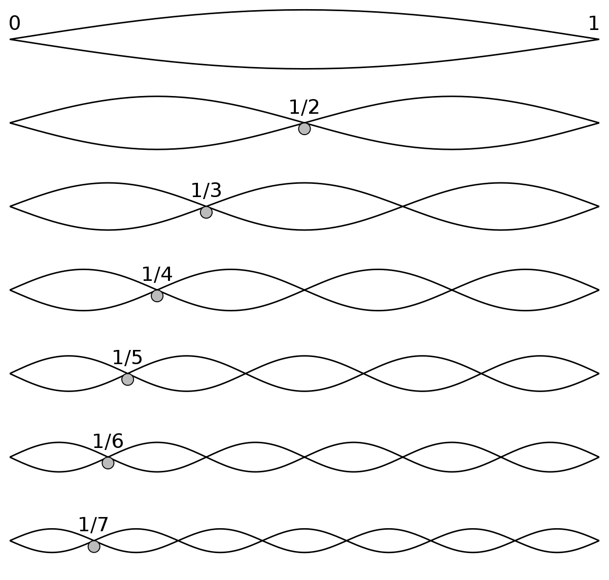
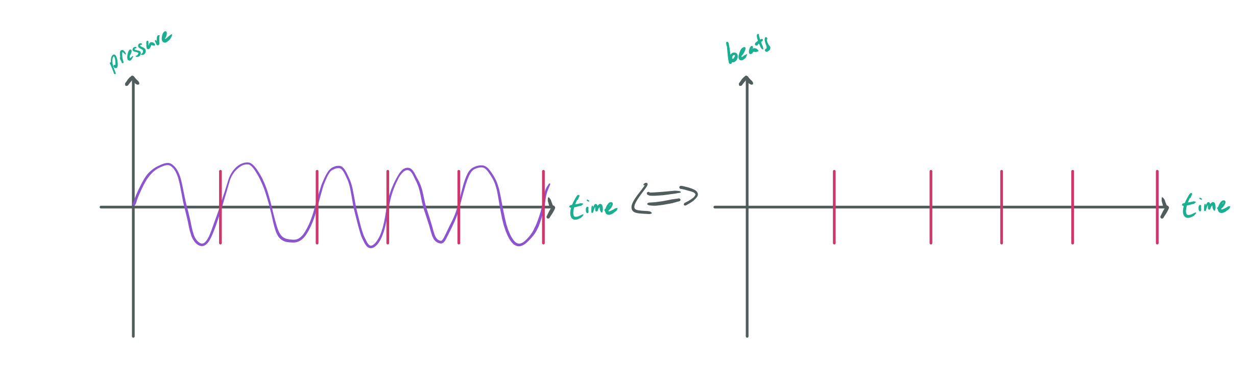
Every harmonic of the second note lines up perfectly with the root note’s even harmonics, making either sound “equivalent” to the ear. Still, this is only part of the picture. A pure pitch an octave above a root will still feel the same, yet they have no harmonic series. How does that work? To explain that, we can switch to looking at consonance from the perspective of the time domain. First, for ease of illustration, I would like to represent a pure pitch as periodic discrete events in time rather than a continuous oscillation like a sine wave.

As doubling frequency is equivalent to halving the periods between cycles, a root pitch and a pitch one octave higher would look like this:

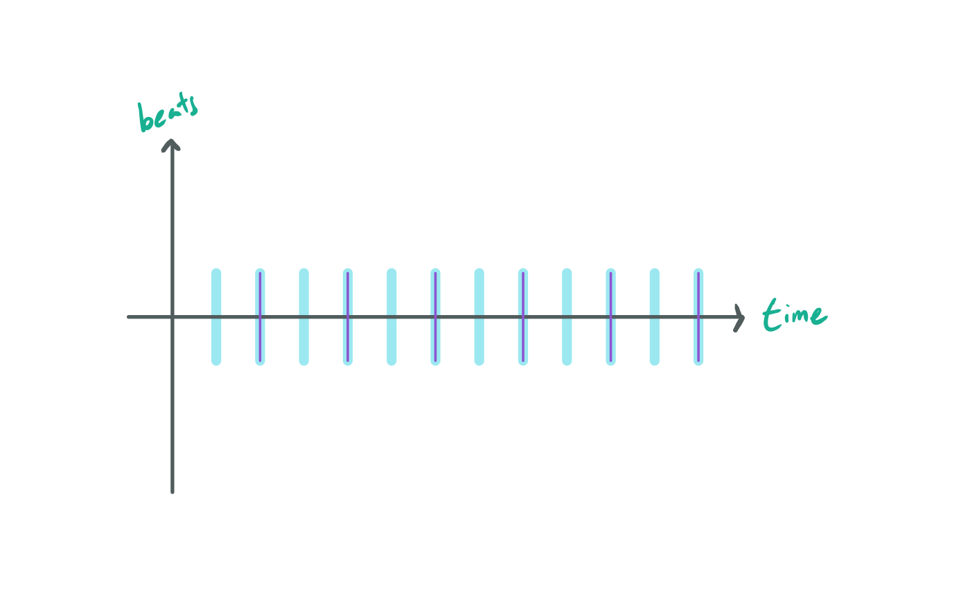
Similar to the frequency perspective where every other harmonic of the octave lined up with the root, every other beat of the octave fundamental pitch lines up with the root fundamental pitch. This pattern repeats every two beats, which is the shortest possible repeating pattern you can achieve in any interval aside from both notes being the same (which would result in the same pattern as the root). To our ears, this sounds like the same note. The doubling of the length of the pattern makes the octave feel less similar than two equivalent notes, but it is close enough that we hear them as the same regardless.

While this does explain the physical intuition for why we perceive the quality of equivalence in the octave, it is also possible for cultures to not perceive it this way. When approaching the foundation of music theory it is also important to keep in mind that these metrics only begin to explain the complex emergent phenomena of music, lest we become overly reductionist. Still, these metrics do provide us with some strong intuition for cultural preferences in identifying intervals. It is most likely not a coincidence that a scale akin to the pentatonic scale (produced from the next type of interval we will learn about) was derived independently by multiple cultures around the world.

A Map of All Intervals

While unison and the octave are fascinating in their own right, as soon as you try to create music using only the octave you will soon realize that nothing interesting will come of it. Music as we know it is produced with not only a variety of intervals, but special orders for them as well we call scales.

Since an interval is simply a ratio of a note to another, and once we reach an octave we have essentially “come home” to the same note we started on, all primitive musical intervals lie somewhere between \(1\) and \(2\). For instance, say our interval is \(3:2\) and we are comparing it to the same interval above our octave \(6:4\). Not only is this note an interval of \(3:2\) away from the octave (a note that is the same as our root), the note above the root at \(6:4\) is one octave from its equivalent at \(3:2\) and will also sound the same. Any structure of intervals we identify between \(1\) and \(2\) can be repeated between any other adjacent pair of integer multiples.

Likewise, there is an equivalency of intervals scaled by any integer multiple. The interval \(3:2\) sounds the same as the interval \(30:20\) as the ratio reduces to be the same (acoustically, this also means that the same interval will sound the same at different root pitches).

It is also worth mentioning that if our metric of consonance is both the frequency perspective of aligning harmonics, and the time perspective of short repeating patterns, any interval representable by an irrational number is not likely to produce a good sounding interval. Rephrased, the harmonious intervals we are seeking for the quality of musical consonance will be rational numbers of the form \(\frac{a}{b}\) (equivalently written as \(a:b\) in music theory, where the convention is set with \(a > b\)).

We have discovered a few basic rules that we can apply to derive the foundation of music theory:

Law of Consonance: Notes sound similar when their oscillations line up frequently in time, or if they share many of the same harmonics.

Law of Rationality: As a corollary to the Law of Consonance, irrational intervals will ensure that either of the necessary properties for consonance will never occur, so pure musical intervals consist solely of rational numbers (or in the case of modern tuning systems, intervals are close to these rational numbers).

Law of Transposition: Any interval (represented by \(a:b\)) relative to an octave is equivalent to the same interval one octave below (e.g. \(6:2\) is equivalent to \(3:2\)).

Law of Reducibility: Any interval \(a:b\) sharing a common factor \(k\) between \(a\) and \(b\) is equivalent to the interval \(\frac{a}{k}:\frac{b}{k}\). (e.g. \(6:4\) is equivalent to \(3:2\))

We can think of these laws as axioms for music theory, but in truth (unlike axioms) we derived them from both physical properties of waves and the psychoacoustic perception of sound. While this makes most of our laws empirical, The Law of Consonance is the hardest one to take at face value as it does require some faith that our ears are able to pick up on the length repeating patterns at audible frequencies. My attempt at explaining the intuition behind this is as follows: Imagine a drummer hitting a drum at a regular interval, then another drum at some multiple of that interval. A \(2:1\) interval will be recognizable, and a \(3:2\) interval would also be recognizable as a polyrythm. In the \(3:2\) case (as we will soon see), the drummer’s pattern repeats every six beats. You can imagine that more complicated patterns that take hundreds of beats to repeat would be nearly impossible to appreciate. It is no coincidence, then, that a major chord is simply a \(4:5:6\) polyrythm sped up fast enough to become audible notes. Rhythm is just harmony at a different time scale. There are deeper reasons for this when speaking only of audible pitches that I won’t give an in-depth explanation here, but going forward let’s assume the Law of Consonance is true.

Running with this idea, let’s start by asking the question “what is the most consonant interval aside from the octave and unity?”. The answer would be quite useful, as any interval less than an octave could be repeated to yield a scale of notes all following this newfound consonance. The answer comes from number theory. The Law of Reducibility restricts our intervals to irreducible fractions and their multiples. When a fraction is irreducible, its numerator \(a\) and denominator \(b\) share no common factors. This property is called coprimality in mathematics. Unlike the concept of primality where a number has no divisors aside from itself and \(1\), coprimality represents an atomic attribute about a pair of numbers.

According to the Law of Consonance, consonance decreases both as less harmonics line up between two notes in their harmonic series, and also as the period of the pattern of their combined fundamentals increases. As you have seen with our exploration with the octave, both of these properties end up with roughly the same picture. The harmonic series provides integer multiples in frequency, and the view as rhythmic beats provides integer multiples in time. Both paths being equivalent, let’s consider the latter case of rhythmic beats. The question of “how often does a pattern of \(a\)Hz against \(b\)Hz repeat?” is actually one that is easy to answer. These patterns will repeat when their beats line up, as the interval between each beat is constant so any instance of beats lining up will yield the same pattern from that point onwards.

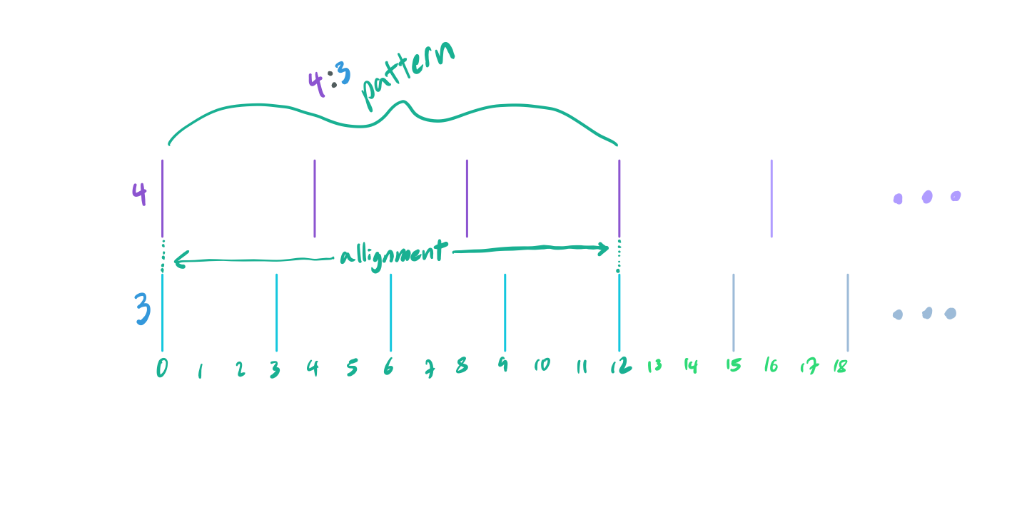
As a side-note, I made the choice to display a rythm of \(4\) as a beat every \(4\) seconds instead of \(4\) beats per second. This makes the allignment easier to visualize, as going the other way around would involve a messy diagram that wouldn’t as easily fit to a grid as the one above does. Either way, it illustrates the interval the same way. Algebraically this is because \(\frac{\frac{1}{b}}{\frac{1}{a}}\) is the same as \(\frac{a}{b}\) or \(a:b\).

Asking “when will the beats line up” is actually the same as asking “what is the least common multiple of \(a\) and \(b\)?”. As we are only talking of irreducible intervals \(a:b\), \(a\) will be coprime to \(b\) (sharing no factors) which means the least common multiple of \(a\) and \(b\) is simply their product \(a \times b\) (it can be no less, as that would imply they did share a common factor). This makes our job easy: we must find the next irreducible interval whose numerator and denominator have the smallest product. The hardest part in this process follows from attempting to make a way of ordering ratios by this property. \(\frac{5}{4}\) is less than \(\frac{3}{2}\), but \(\frac{3}{2}\) corresponds to a more consonant interval as the product of the numerator and denominator \(6\) is less than \(20\) (the product of numerator and denominator of \(\frac{5}{4}\)).

What if we started by considering increasing denominators, listing out all fractions and removing ones that either are reducible (from the Law of Reducibility) or equivalent to ones we have already listed (also from the Law of Reducibility)? To make things easier, we can enumerate all rational numbers from \(0\) to \(1\) instead of from \(1\) to \(2\). I think for most it is easier to think about ratios like \(\frac{2}{3}\) instead of ones like \(\frac{3}{2}\) as the latter is greater than one and “feels” less like a ratio. We can simply invert any ratio we find, as inverting a ratio does not change the product of its numerator and denominator.

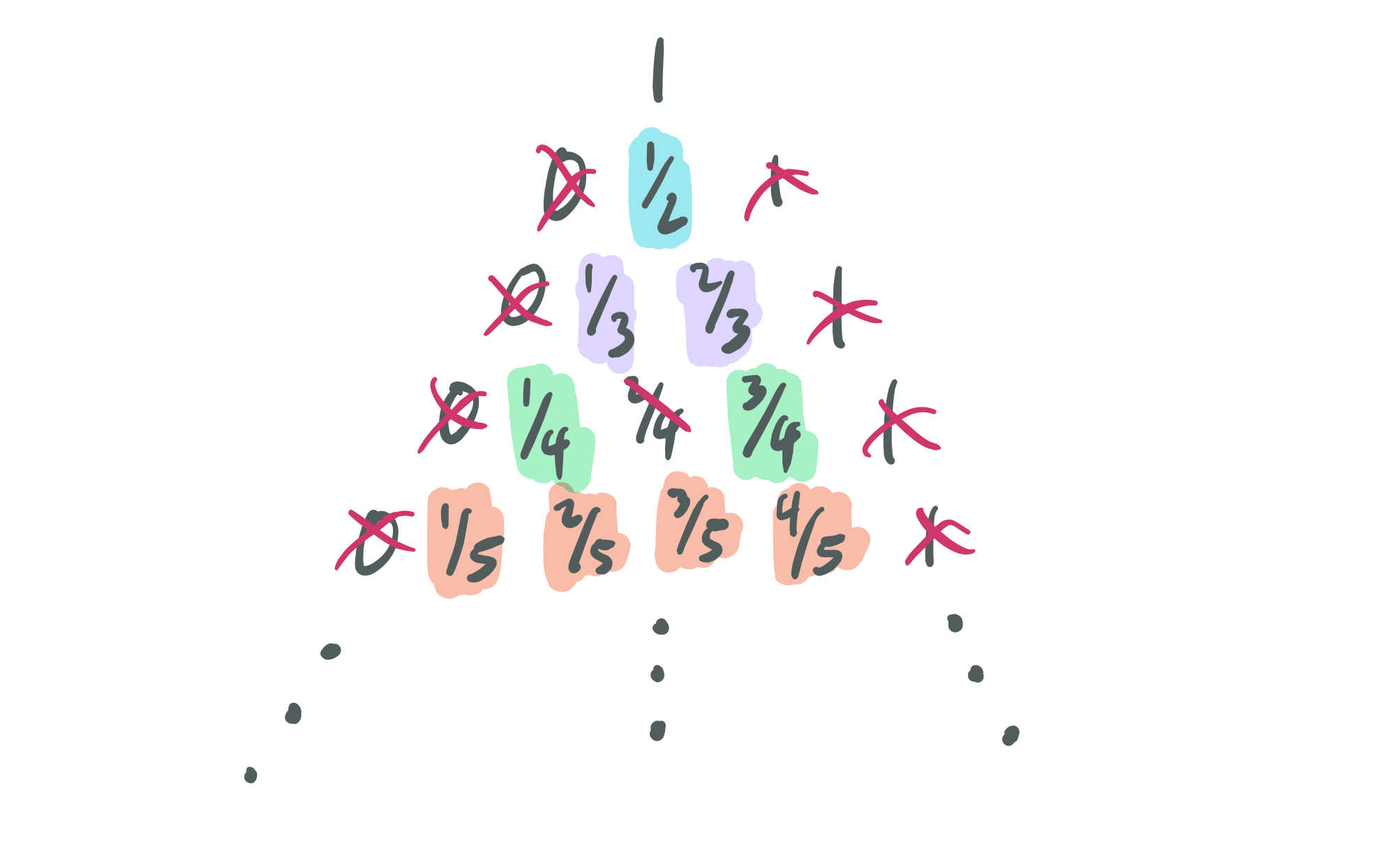
Once again, mathematics has a name for this process and the terms it generates: the Farey Sequence. The only difference is that the Farey Sequence does allow for repeated terms as we generate new rows. This means that for the sixth order, the inclusion of \(\frac{2}{6}\) will be allowed and be written as \(\frac{1}{3}\). Each successive iteration of the Farey Series also includes the last, but adds the mediant between each pair. This yields a definition similar to the one we derived, but unique in its own way: “The \(n\)th Farey sequence contains all irreducible fractions less than \(1\) with denominators less than \(n\)”.

\[ F_1 = \huge\{\normalsize \frac{0}{1}, \frac{1}{1} \huge\} \] \[ F_2 = \huge\{\normalsize \frac{0}{1}, \frac{1}{2}, \frac{1}{1} \huge\} \] \[ F_3 = \huge\{\normalsize \frac{0}{1}, \frac{1}{3}, \frac{1}{2}, \frac{2}{3}, \frac{1}{1} \huge\} \] \[ F_4 = \huge\{\normalsize \frac{0}{1}, \frac{1}{4}, \frac{1}{3}, \frac{1}{2}, \frac{2}{3}, \frac{3}{4}, \frac{1}{1} \huge\} \] \[ F_5 = \cdots \]

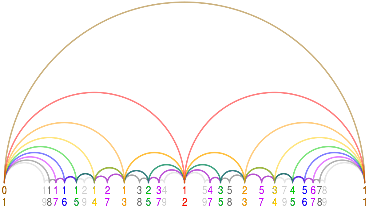
This is an powerful abstraction. In a way, it allows us to select a certain amount of allowable complexity (bounded by the denominator) and produce all possible ratios with that property. In fact, you only need to construct the eighth Farey Sequence in order to produce all intervals we use in Western music. If you were to stop at five, you would only exclude the major seventh and the major semitone (which also explains why those two intervals are generally considered so discordant compared to the others). We can also plot these sets different paths from \(0\) to \(1\) along rational stepping stones:

To recover what intervals are possible as ratios relative to a root, start with any Farey Sequence and only consider any ratios larger than \(\frac{1}{2}\). Remember that we inverted the convention of making the numerator larger than the denominator, so to go back to where we were before we can invert the remaining ratios. We chose \(\frac{1}{2}\) as a start, as \(\frac{1}{\frac{1}{2}} = 2\). Likewise, the last element of any Farey sequence will be \(1\), which inverted will still be \(1\). This is why we eliminated any ratios less than \(\frac{1}{2}\), as their inversions would be greater than \(2\), which would be above the octave. Lastly, we have to reverse the order as the inversion has flipped our ascending order to a descending one. For example, assuming we are using \(F_3\):

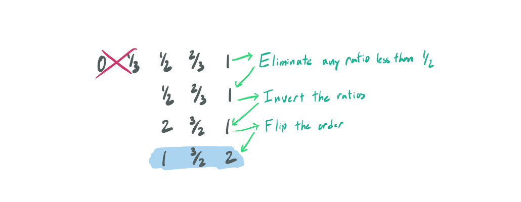
This means that the next most consonant and harmonious interval is \(3:2\), otherwise known as The Perfect Fifth. Any musician will most likely agree that this interval sounds very good. So good, in fact, that the majority of scales musicians work with are generated from this interval. The Circle of Fifths is proof of this, and serves as one of the most useful tools in music theory for navigating scales and harmony. Every step along this circle is roughly a perfect fifth.

Vineyards

We’ve come a long way in this exploration into music theory, so before we continue I wanted to explain how this ties in with the patterns in vineyards and orchards. If you have never seen this derivation before, it may not seem obvious how these two worlds are in fact different sides of the same coin. First, realize that a vineyard or orchard consists of posts placed at regular intervals. For the sake of example, assume the posts are distributed along a grid with equal gaps both horizontally and vertically. What are the gaps that we see as we stand on the edge of the orchard and peer in? It turns out that is an extremely difficult question, and it would be easier to start by asking “What angles of my view into the orchard are obstructed by vines or trees?”.

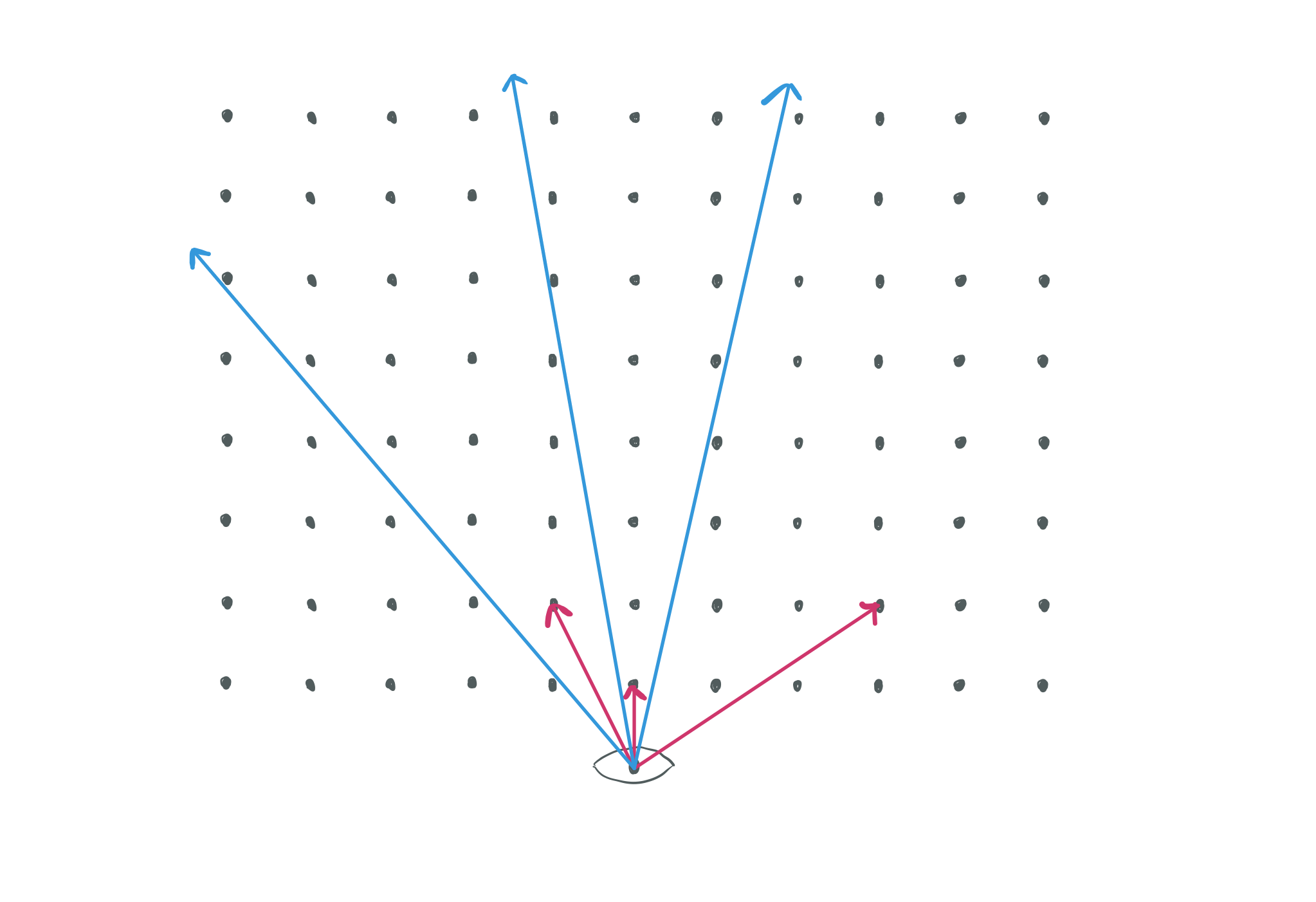
Don’t see it yet? The pattern is easier to see if I add a coordinate system where you are standing at \((0,0)\), and the posts are all placed at integer coordinates away from you.

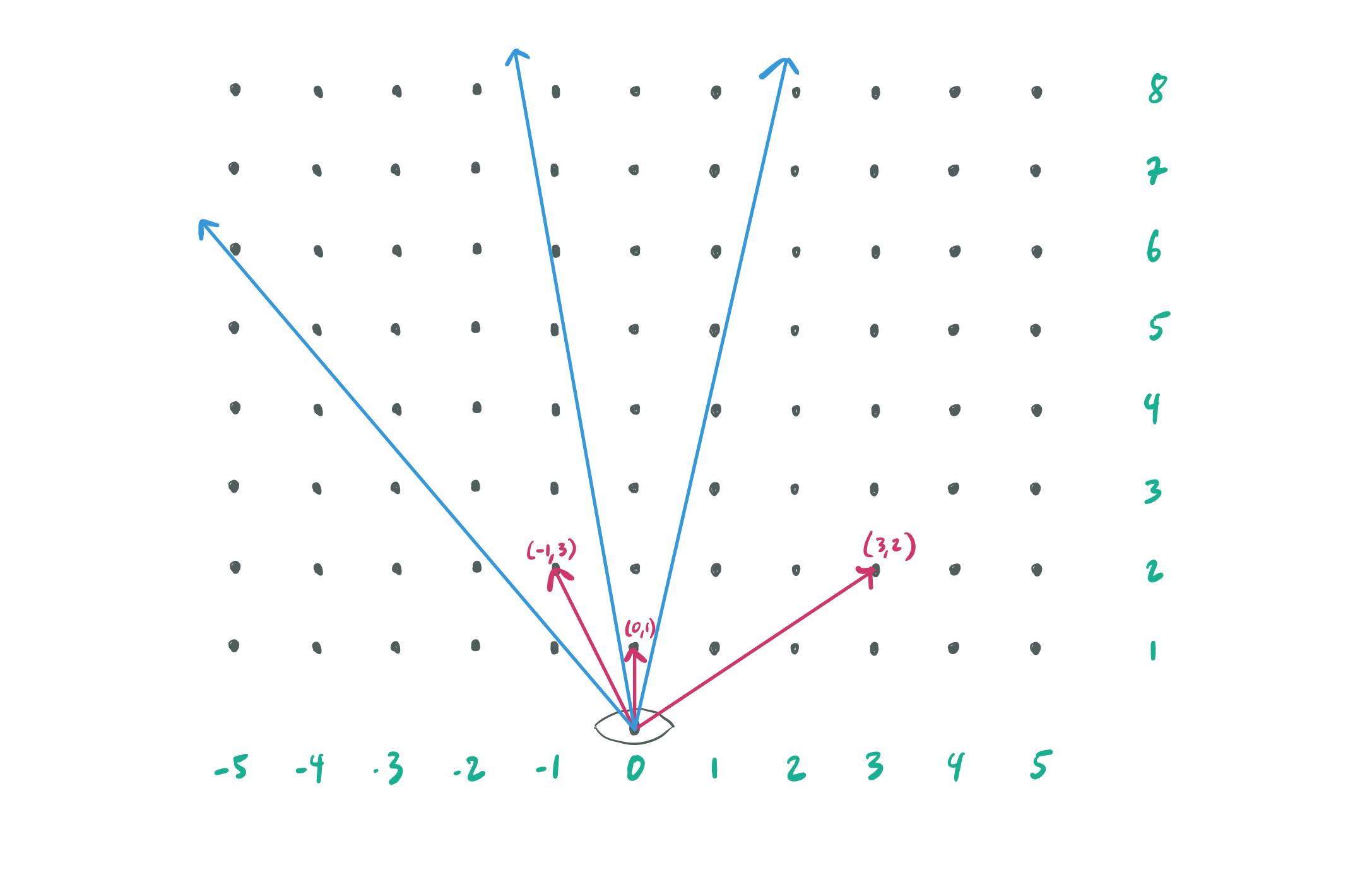
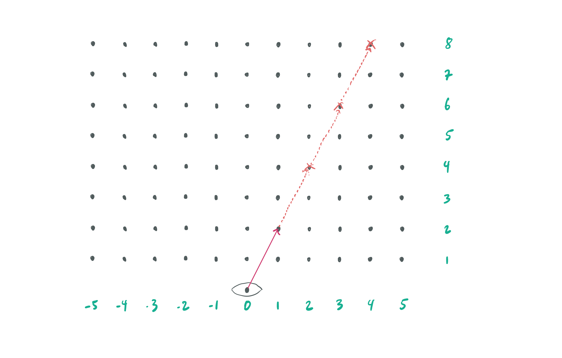
Consider the representing any ratio \(\frac{a}{b}\) instead as coordinates \((a, b)\) and you will soon see that the vineyard has vines corresponding to rational numbers! Not only that, but the concept of irreducibility is actually encoded in this view as if there is a vine at \((a, b)\), it will block the vine at \((2a, 2b)\) (and any integer multiple higher).

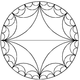
Also, as the denominator can correspond to the horizontal coordinate, as you sweep your vision from left to right the vines you see will be in the same order as in the Farey Sequence. This means that every vine you see corresponds to a valid harmonic interval, and the vines closer to you represent more harmonic intervals that possess more consonance than the ones further away. Looking into the vineyard, your view would look something like this (red posts are two away from the center):

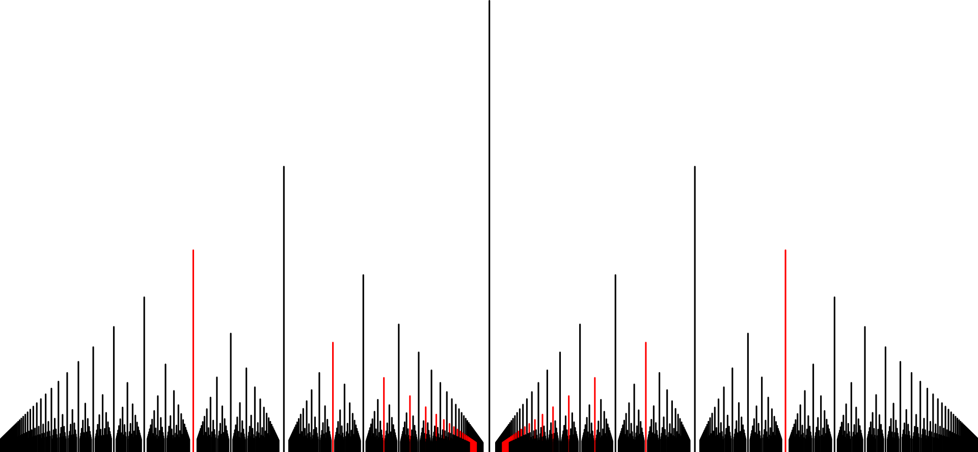
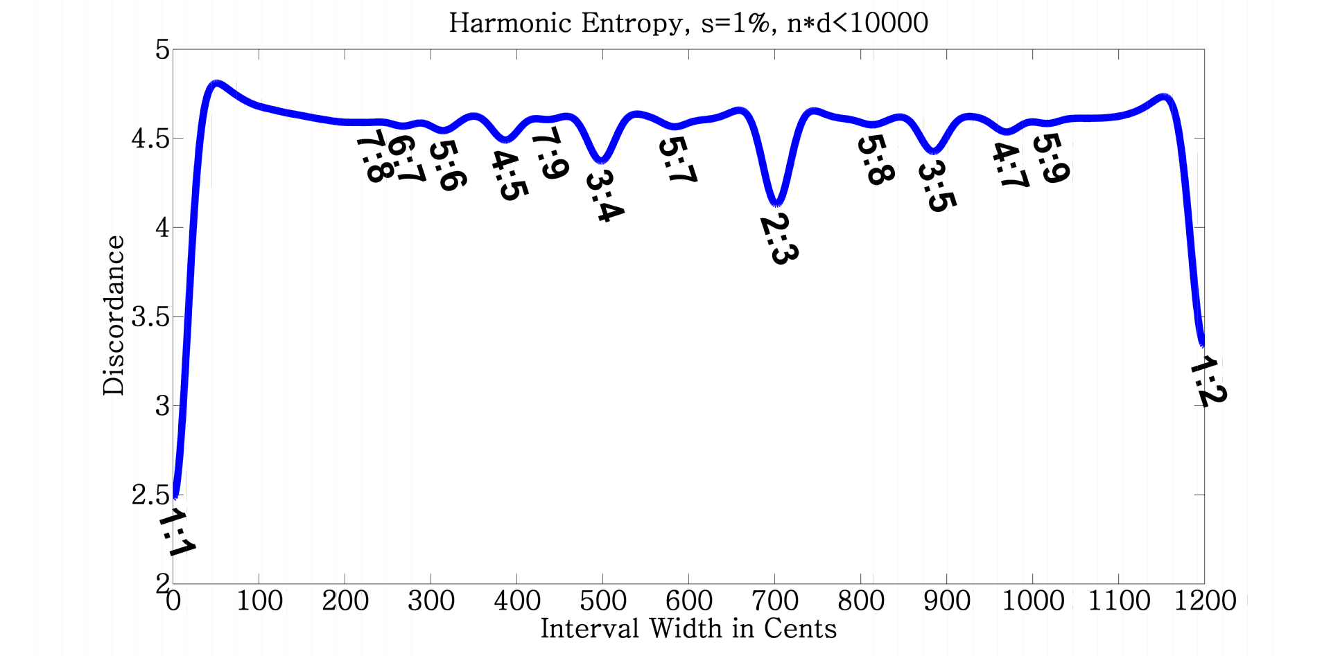
This structure is called Euclid’s Orchard and (like many other structures in math and number theory) relates closely to the Farey Sequence. You’ll note that more consonant intervals have larger gaps around them. An alternate view is that the gaps we see in the vineyard correspond with more consonant intervals. The Theory of Harmonic Entropy is built on this view, and examines the question “If I choose a random direction to look, and if each post has a small diameter, how many posts on average obstruct my view in that direction?”. This turns out to be equivalent to looking at the Shannon Entropy of the vineyard. Basins of low entropy mean that there aren’t many vines around that direction, which then corresponds to more consonant intervals.

The most well-used intervals emerge from the gaps. A major chord is made of the perfect fifth, and the next most consonant interval (the major fourth). Here are some notable intervals and the gaps they correspond to:

• \(3:2\) - Perfect Fifth
• \(4:3\) - Major Fourth
• \(5:4\) - Major Third
• \(5:3\) - Major Sixth
• \(6:5\) - Minor Third
• \(8:5\) - Minor Sixth
• \(7:4\) - Harmonic Seventh
• \(7:5\) - Tritone

It was easy enough to find where posts were located. Gaps, however, are a different story. Gaps exist where your line of site will never hit a vine, which means that it corresponds to an irrational number (one that cannot be represented as a ratio of two integers). The curious thing about this fact is that rational numbers are dense in the real numbers. This means that for any two rational numbers \(x\) and \(y\) you can always find another ratio \(z\) greater than \(x\) and les than \(y\) (which is to say that \(z\) is between \(x\) and \(y\)). This means that (in an infinite vineyard) for any point where you can see through the vineyard, you may find a vine arbitrarily close to your angle of vision. In this sense, an infinite orchard has no gaps in it whatsoever. Going back to music theory, this means that any number is arbitrarily close to a musical ratio! The crux is that as you approach irrational numbers, the numerator and denominator grow in size substantially meaning any ratio close to an irrational one is likely to be dissonant.

We just learned that the gaps we see in vineyards and orchards are largely due to their finite size. If the rationals are dense, why do we see gaps at all? Why does it seem like there are sections where rational numbers are “more dense” than others? If you find the answer, don’t tell me, write a paper on the topic and receive a million dollars and international notariety as the most accomplished mathematician who ever lived. Understanding the pattern of these gaps is in fact equivalent to understanding the Riemann Zeta Function, which is the topic of The Riemann Hypothesis: a conjecture that is among ten problems that carry a one million dollar bounty for their solution.

Even though we don’t understand these gaps, an interesting fact is that if you were to randomly pick a direction to look in the vineyard the probability that your vision would be obstructed by at least one vine approaches \(\frac{6}{\pi^2}\) as the orchard grows larger in size. This ends up being equivalent to the famous Basel Problem, which has many satisfying solutions, one of which is evaluating the Riemann Zeta function at 2: \(\zeta(2) = \frac{\pi^2}{6}\). Conceptually the “\(2\)” represents the two integers being picked for the ratio.

For fun, I also wanted to share what this vineyard would look like in three dimensions. Thankfully, we have a game today that makes this visualization not only easy but actually one that people have stumbled across by chance: Minecraft. There is a map you can download that has random blocks from the game distributed at regular intervals in a three dimensional lattice (sound familiar?). This is what it looks like:

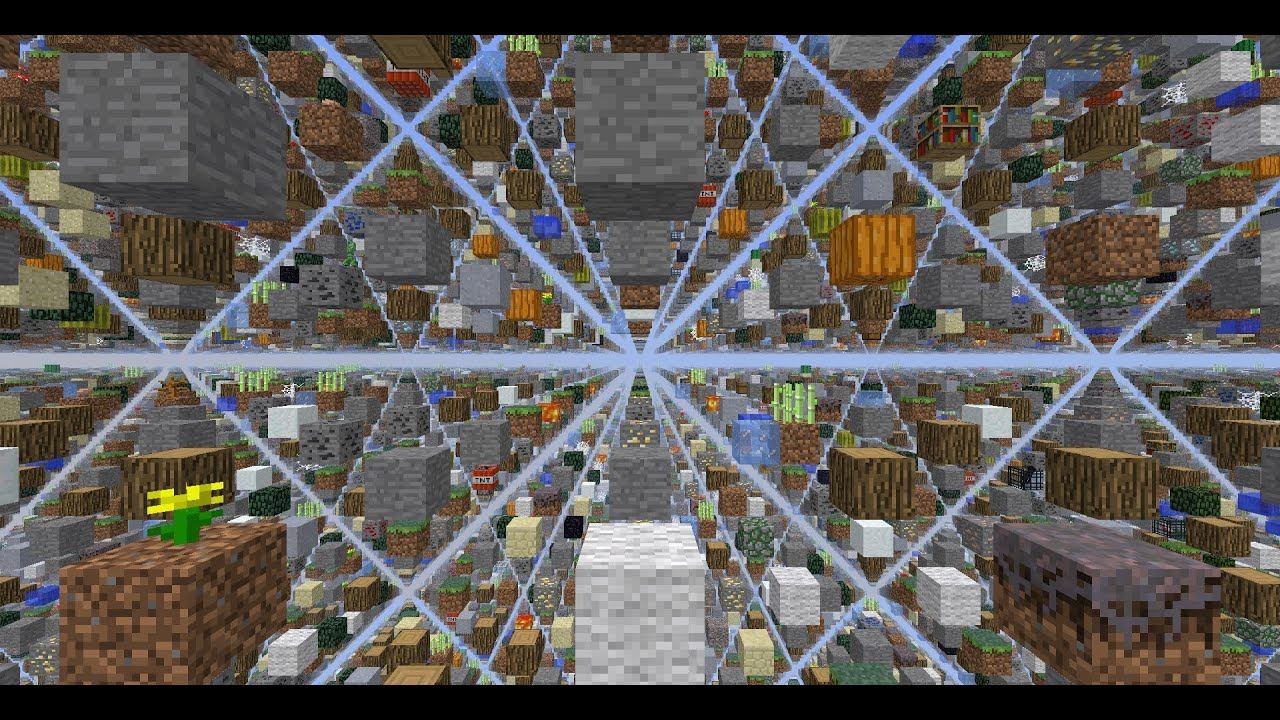
I invite you ponder on how this relates to chords: pairs of intervals involving three terms instead of just two.

Further Connections

In my explorations, I also came across how the major scale was derived from the perfect fifth, and how scales are generated by rotating the major scale about all seven of its degrees (called modes). Maybe some time soon I can write up another post on how scales are generated, how they relate to the Fibonacci Sequence, and some history as to the compromises that led us away from rational numbers towards 12-Tone Equal Temperament. Ironically enough, all intervals on a modern piano, guitar, horn, and most instruments correspond to irrational intervals (albiet very very close to their rational counterparts).

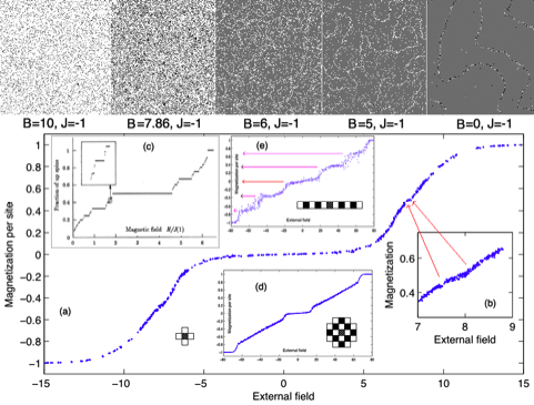
For now, I will leave you with a list of other surprising places the Farey Sequence shows up: The Ising Model - This model of the physics underlying magnetism in permanent magnets shows how the Farey Sequence identifies states where particles exchibit self-organized criticality and produce ferromagnetism.

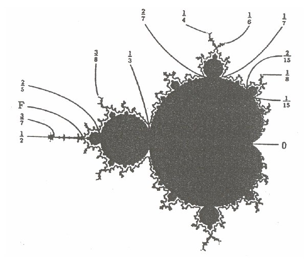
The Mandelbrot Set - This is one of the earliest computer generated fractals. It shows up often in the of the study of Dynamical Systems along with Chaos Theory. The Farey Sequence corresponds to critical values of angles on the exterior of the set (source).

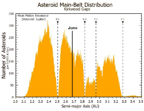
Asteroid Distribution With Respect to Orbital Period - If you plot the amount of asteroids in orbit around a central body in terms of the period of another orbital body, there will be gaps in the asteroids proportional to terms in the Farey Sequence.

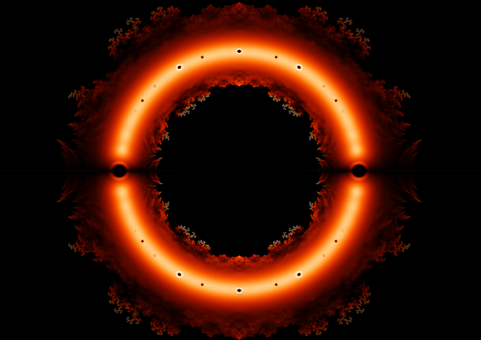
The Pattern of Gaps in Polynomial Roots - I don’t yet have confirmation that this does involve the Farey Sequence, but the similarity is so close it’s hard to not mention it. This fractal is produced when you make a heatmap of the roots to millions of integer-coefficient polynomials. The holes in the main band (the unit circle) seem to correspond to Transcendental Numbers (my reasoning for this is that they would not be included in this set, and gaps would form similar to how gaps form in the rationals in the case of Euclid’s Orchard). This is an open question for me, and I’d love to understand why these holes exist where they do.

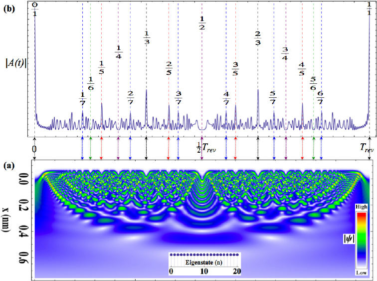
Quantum Oscillators - Various Eigenstates of quantum oscillators correspond closely to the Farey Sequence.

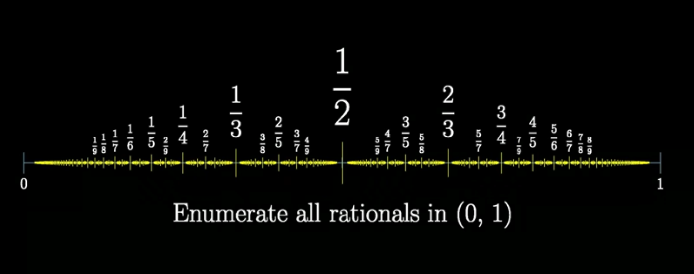
Measure Theory - Three Blue One Brown’s video on measure theory actually gave me much of the intuition for what I’ve shared in this post. And while I think Grant does not explicitly mention the Farey Sequence, he produces a cover of the rational numbers using the same concept.

Approximating a Sphere - When you approximate a sphere using voxels (cubic pixels) many cuts begin to appear as you use smaller and smaller voxels.

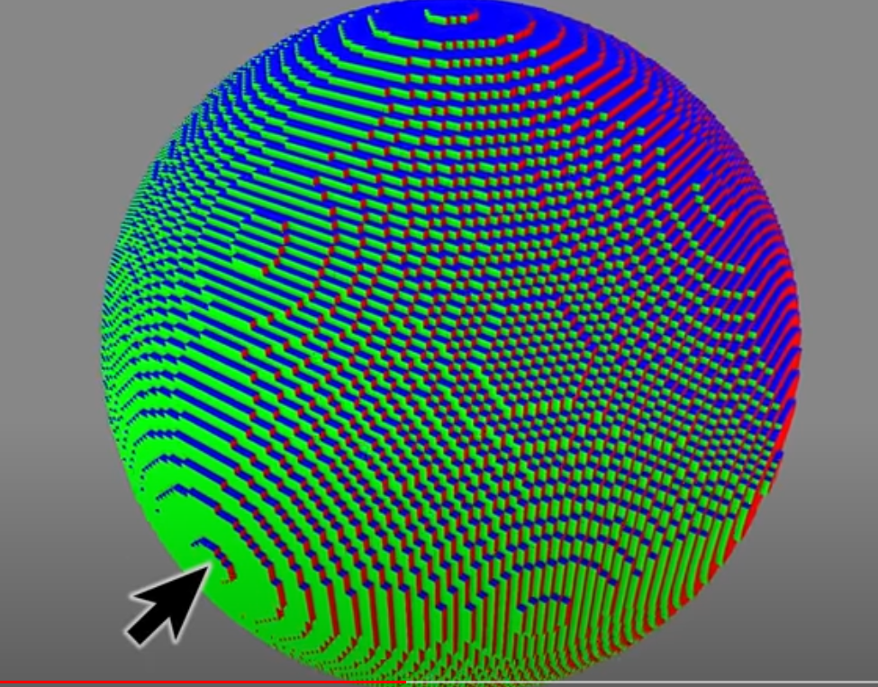
These cuts correspond to the Farey Sequence mapped circularly instead of in the plane:

Miller Index - The Miller Index is a way of assigning labels to different planes in Crystallography. This is very similar to the sphere example I just mentioned.

Thank You

Thanks for coming along for this journey with me! There are no doubt many more instances of the Farey Sequence showing up in our lives, in music, and in the universe. It’s a gorgeous structure that reminds us how disparate topics can be intimately connected behind the curtain.