Digital Astronomy with Cellular Automata

In my last post, I shared my journey through understanding the link between entropy, thermodynamics, evolution, computation, and mathematics. At the end, I shared some preliminary research on using entropy/complexity to classify the behavior of Cellular Automata (CA) and perhaps pave a road to finding more universal CA (those capable of computation). At that time, I only had a handful of samples which, albeit showing promise, fell short of demonstrating concrete results.

I am incredibly excited to share that I have now run my simulations on every possible Life-Like Cellular Automaton rule (a total of 262,144 rules), and it shows some great potential in classifying every rule based on its emergent behavior. Not only that, but this method establishes what appears to be a strong metric for finding “islands” of rules that have similar behavior.

This is exciting news, because past classifications of even elementary CA such as the semi-totalistic Moore neighborhood variety (called the Life-Like CA) have either required generalizations that are computationally intractable to ascertain, or required a great deal of manual filtering and edge-case handling in order to separate sets of rules into classes.

Abstract

Stephen Wolfram (one of the biggest researchers in CA) proposed a four-level classification scheme for one dimensional cellular automata. He later extended these definitions to include two-dimensional cellular automata like the Life-Like CA we are looking at here. The classifications are:

1. Evolution leads to a homogeneous state.
2. Evolution leads to a set of separated simple stable or periodic structures.
3. Evolution leads to a chaotic pattern.
4. Evolution leads to complex localized structures, sometimes long-lived.

But, as mentioned in this post regarding some caveats about these classifications, gliders have been found in all four of these classes. This is problematic because gliders are one of the most essential parts of data transmission in machines built inside of CA, so the four classes may not be enough to identify the presence or absence of a universal CA. Also, it has been shown that, given a rule, finding which class a CA belongs to is an undecidable problem (for one-dimensional CA at least, but I would imagine the argument abstracts well to any Cartesian dimension).

My goal here was to focus on dynamic classification of the emergent properties of any given CA given its rules. By not subscribing to manually generated labels on classification, we can instead focus on developing a metric of similarity. In this sense, each rule becomes its own “class” and you can find rules that are sufficiently close in behavior to be considered the same class. Geometrically, this would be an analysis of CA by way of clustering.

The difficult part, of course, is developing a representation of a given rule that would allow for clustering. I settled on producing a curve of the Kolmogorov complexity across the generations of the automaton’s universe. My inspiration for this approach came from a few core concepts. First, that entropy and complexity looked like valid metrics to measure the emergent behavior of a system and its potential for self-organized criticality. My reasoning behind this intuition is that structure typically implies order, and order implies either repeating patterns or extension of structure that can be derived from existing structure. Kolmogorov complexity would capture the amount of bits required to express this structure. I later learned that this view is not a new one, as Wolfram took a similar approach in examining the procession of spacial and temporal entropy in his research on one-dimensional CA.

In a addition to the convenient dualistic simplicity of studying life-or-death CA, the grid of an automaton can be interpreted as a bitmap image. Image compression is (unsurprisingly) adept at finding something close to the smallest possible representation of an image, and PNG compression does it without loss of information. Image compression asymptotically approximates Kolmogorov Complexity up to a constant dependent on the compression algorithm. Therefore, as the compression algorithm is the same for each measurement, we have a viable pipeline for estimating the Kolmogorov complexity of each state of the CA universes we encounter. If we wish to relate all of this back to entropy, we can do so. Entropy is the expected value of Kolmogorov Complexity in this context, so this data will be useful for that as well.

In order to get an amortized generalization of each rule, I started from random initial states of the universe with each cell having an equal probability of starting in any of the possible states. I then ran simulations for hundreds of generations with multiple random initial conditions and found the average complexity at each step. Other researchers looking into the general behavior of CA have taken this approach of random initial state and it seems to be a valid way to capture their behavior.

Lastly, I chose to study only Life-Like CA. These are the semi-totalistic CA rules that only depend on the Moore neighborhood of each cell. This made the search space something that I could simulate in reasonable time, given that it only had around a quarter million possible rules (even though it still took two weeks to generate all of the data).

The result of these simulations were 262,144 records of the average complexity in bytes of the board of all possible Life-Like CA. Each record had 256 samples, each record was averaged from 10 runs, and each rule was run with a board size of 100x100 cells.

Using UMAP, a Digital Telescope

Obviously, no one has the time to go through the graphs of over a quarter million samples, so I needed to find a way to classify the results. Recently I have been infatuated with the UMAP algorithm. It has the ability to compress data with thousands of dimensions into a lower dimensional space (in this case 2D or 3D) while still preserving structures/features in the data. It is a remarkable feat of algebraic topology that deserves more awareness of in the scientific community.

When first learning about dimensionality reduction algorithms such as UMAP or tSNE, I was extremely skeptical of their efficacy. It seemed impossible to retain structure when losing that many dimensions. What made their usage click for me was the knowledge that, even if your data lives in a space that has thousands of dimensions (called the ambient space), there is a very good chance that the local dimension of real-world data is of much lower dimension than this. The goal, then, of UMAP is to preserve the structure found in the data by finding a good manifold to embed it into. For further understanding on this topic, check out the presentation that Leland McInnes (the creator of UMAP) gave on his algorithm.

In a sense, UMAP is a digital telescope that lets us look at constellations of high-dimensional data that we have never had the ability to visualize before. Algorithms like tSNE have worked in similar ways in the past, but UMAP is the first algorithm to be efficient enough to run on data with thousands of dimensions using something as prosaic as a laptop and a dream. This is to say that UMAP scales incredibly well, especially when compared to what is already out there.

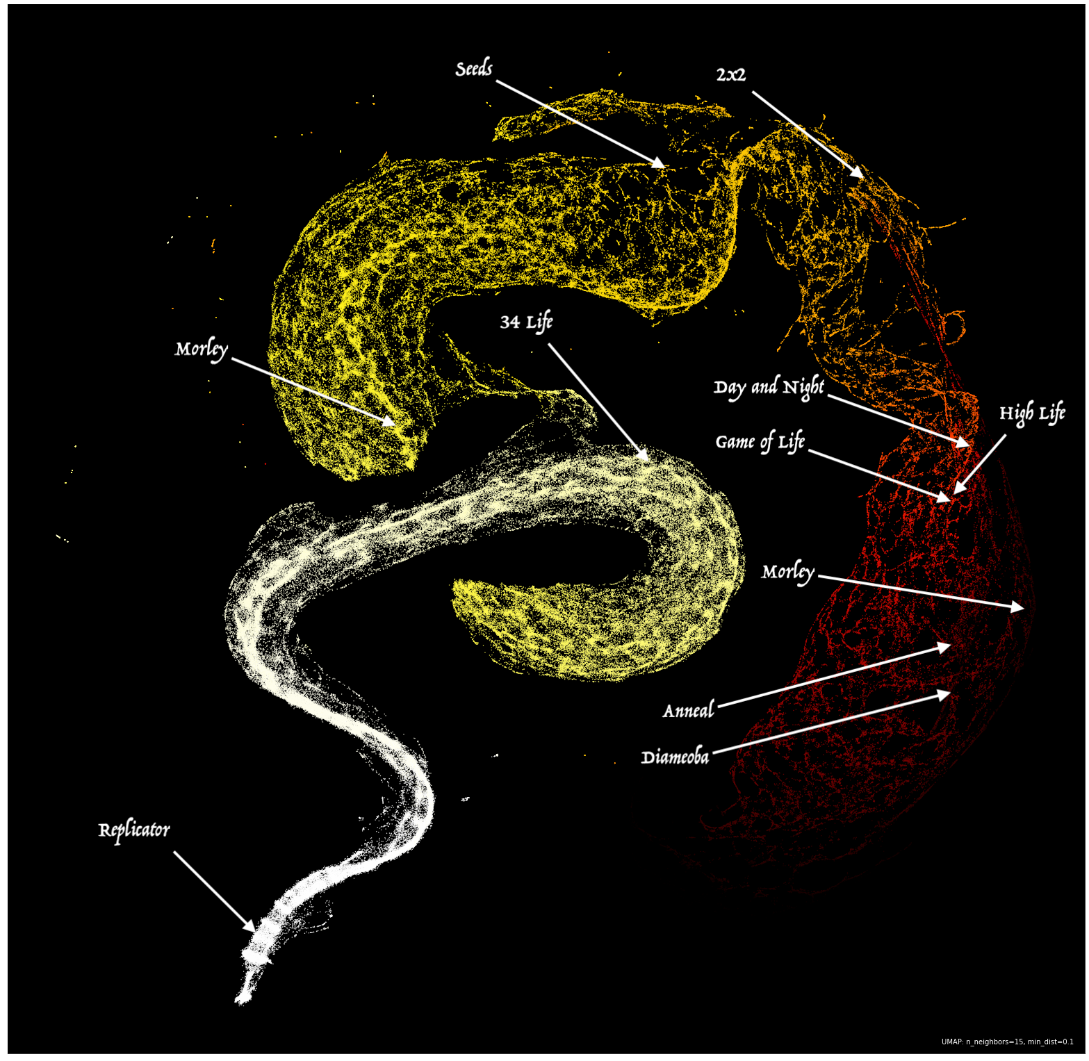
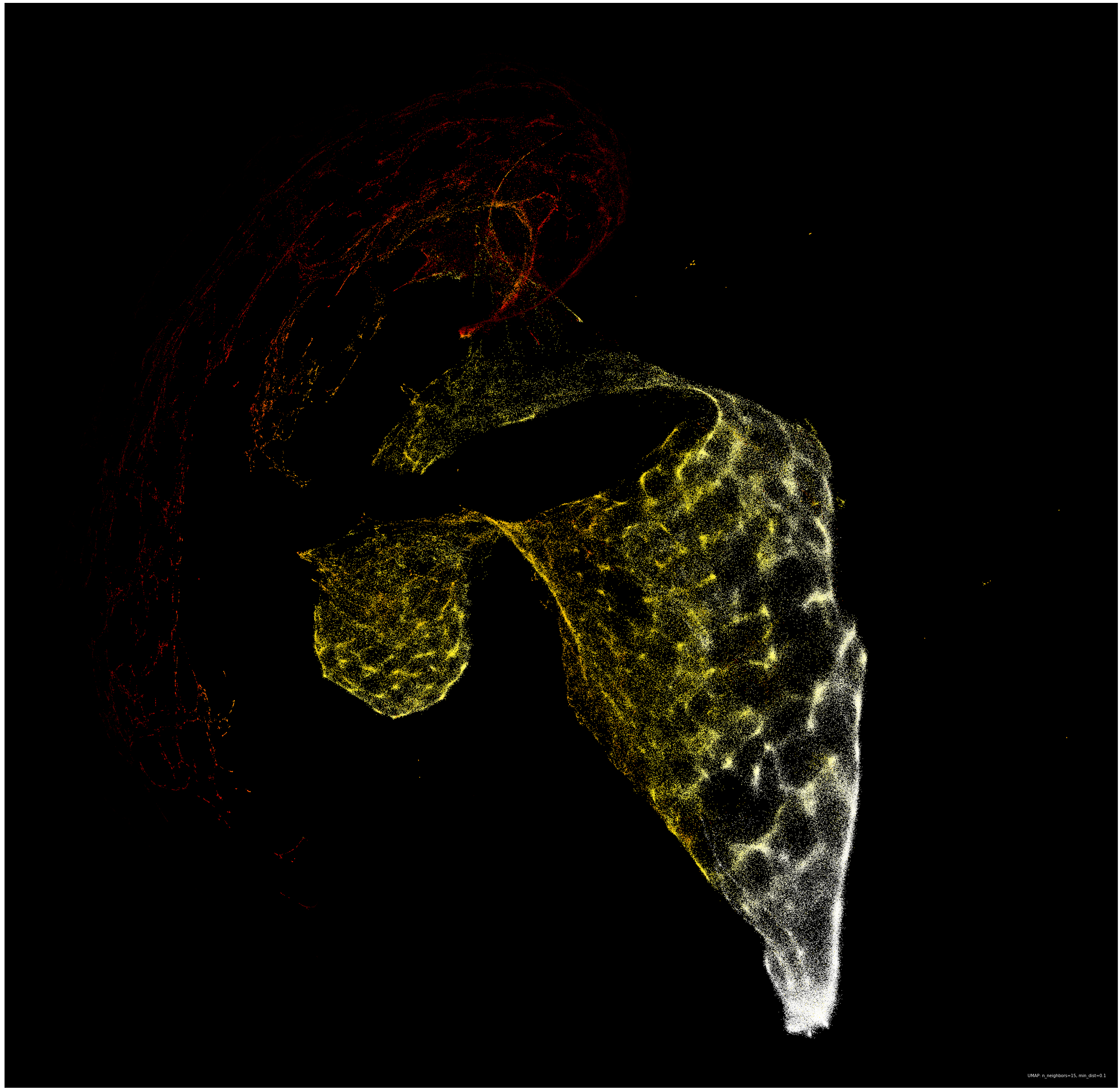
Armed with UMAP, I fed the algorithm all 262,144 vectors (each with 256 dimensions, one for each complexity snapshot) and patiently waited for the embedding to complete. After fifteen minutes of my laptop revving up my fans, I had my first snapshot of the overarching structure of the Life-Like CA (points are colored by the average forward difference between each complexity snapshot):

(High-Res Version)

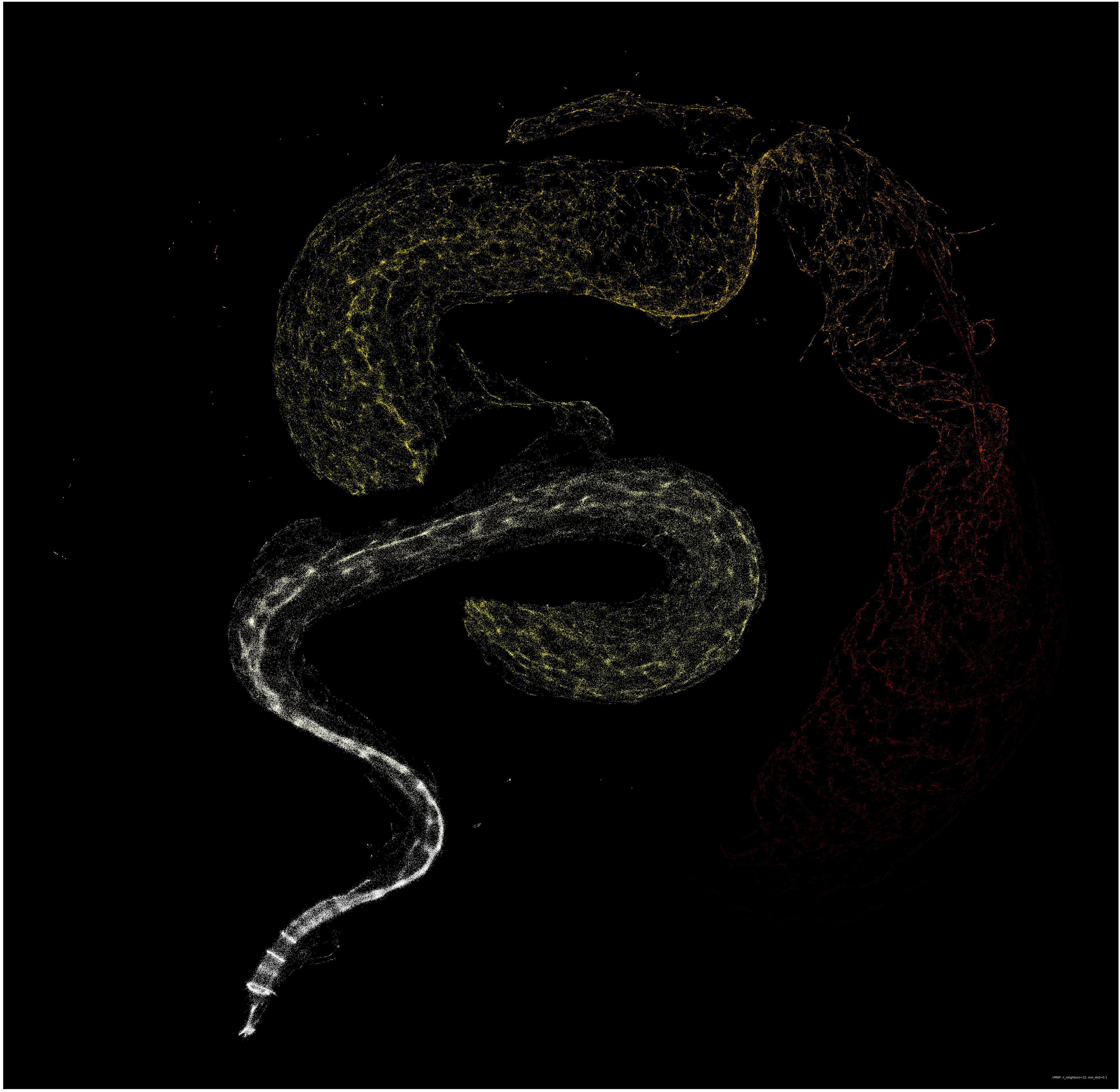
There it was, the massive Hertzspring-Russelesque serpent hiding in the structure of emergent complexity in automata. It is important to note that compressing dimensions can make parts of the data look separate in the embedding, even though they are connected in the ambient space they came from. It would be reasonable to assume that the serpent is one continuous entity, and the “jump” in the center was a result of the embedding.

While beautiful, this representation would not mean much if it did not accomplish the goal we set out to achieve: a metric for classification of rules that behave in similar ways to a given starting rule. Starting from the Game of Life, I began examining nearby rules and found that the metric did indeed yield other rules that produced uncanny behavior.

Rules Close to the Game of Life (B3/S23)

B3/S23	B3/S013	B38/S013	B38/S238

Rules Close to Day and Night (B3678/S34678)

B3678/S34678	B36/S01456	B3678/S01456	B3567-S01478

Rules Close to Anneal (B4678/S35678)

B4678/S35678	B468/S035678	B0123578/S0124	B46/S035678

Rules Close to Maze-Finder (B138/S12357)

B138/S12357	B124/S123467	B0124/S0123467	B038/S012358

What is fascinating about this embedding is that it extends the idea of Stephen Wolfram’s four-level classification of CA to a continuum that can be embedded in as many dimensions as you see fit. CA classically known for supporting persistent structures and gliders such as Game of Life, Day and Night, and High Life exist in the middle of the serpent where the average difference is on the edge of chaos. CA that burn through complexity at a higher rate such as Morley, Anneal, and Diamoeba are far out on the tail of the serpent, along with many rules that result in universes that either die out quickly or fill the whole board with live cells (two low-complexity attractors). Meanwhile, rules like Replicator (which duplicates existing structure) exist in the head of the serpent where complexity stays roughly the same throughout the generations. Rules at the head seem to tend very quickly towards chaos, an apt opposite to the rules found in the tail.

Caveats and Room for Improvement

You might notice that for the Anneal CA that there was an example that behaved like Anneal but oscillated between black and white states every generation. This was one of the most fascinating parts about this structure for me. Rules that normally would not be classified together clearly had similar behavior, even though they had different ways of expressing it.

This didn’t always work out for the best though, and there were cases of “close” rules that had obviously different behavior. I think this shows that this complexity metric either requires more resolution in the samples, or that some types of behavior are not adequately described by the procession of complexity alone.

One major improvement that I could see benefiting this model would be a transformation on the data that would be resilient to translations in the complexity curves. For instance, perhaps one CA immediately takes a dive in complexity following one behavior, and another with similar behavior is just slightly slower to hit that tipping point. Both curves would look nearly identical, save for the latter one having the sigmoid-like decrease in complexity occur later in the curve. If you were to translate the first curve forward, or the second curve backward in time you would have a better metric for joining complexity like that.

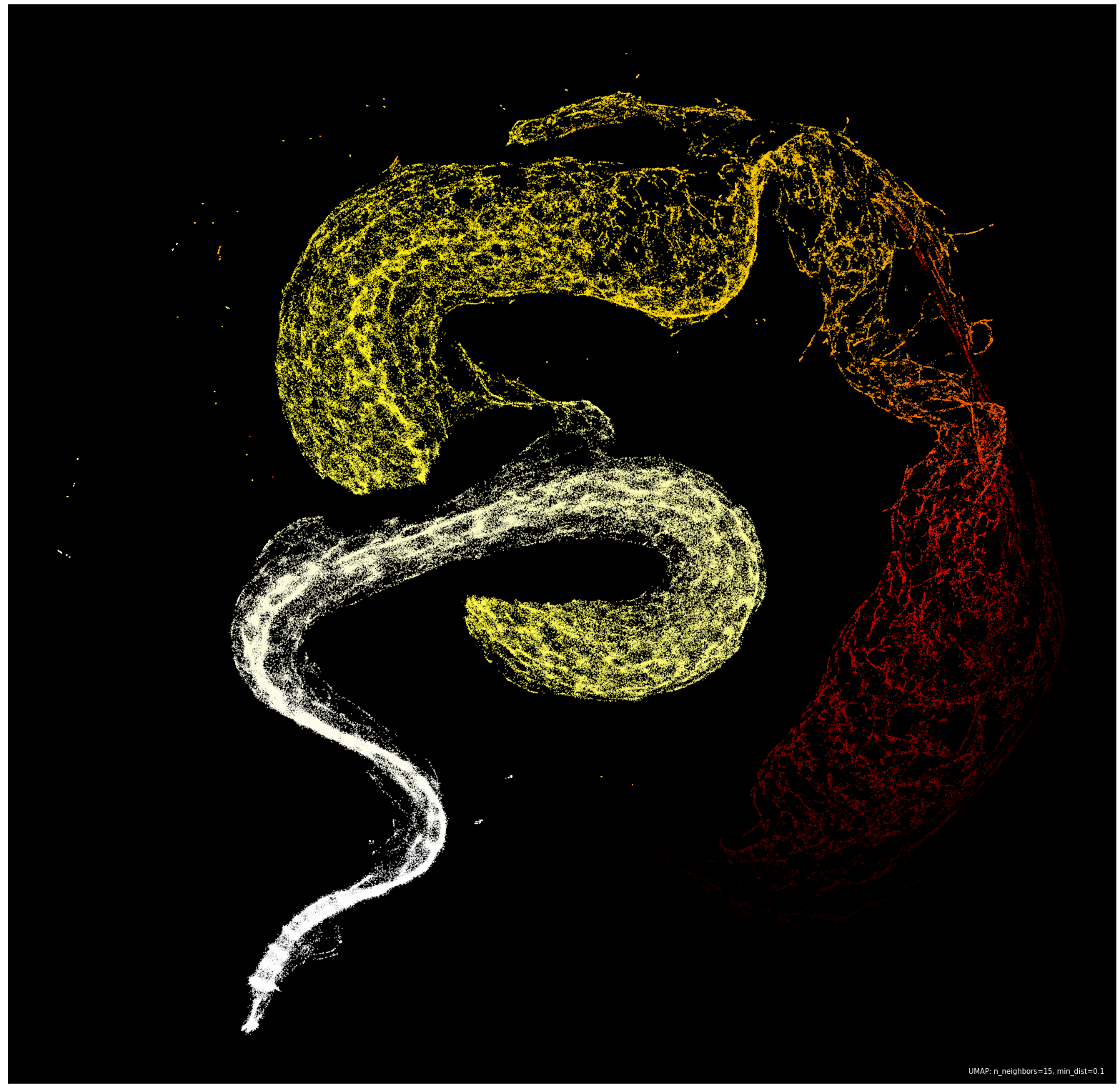
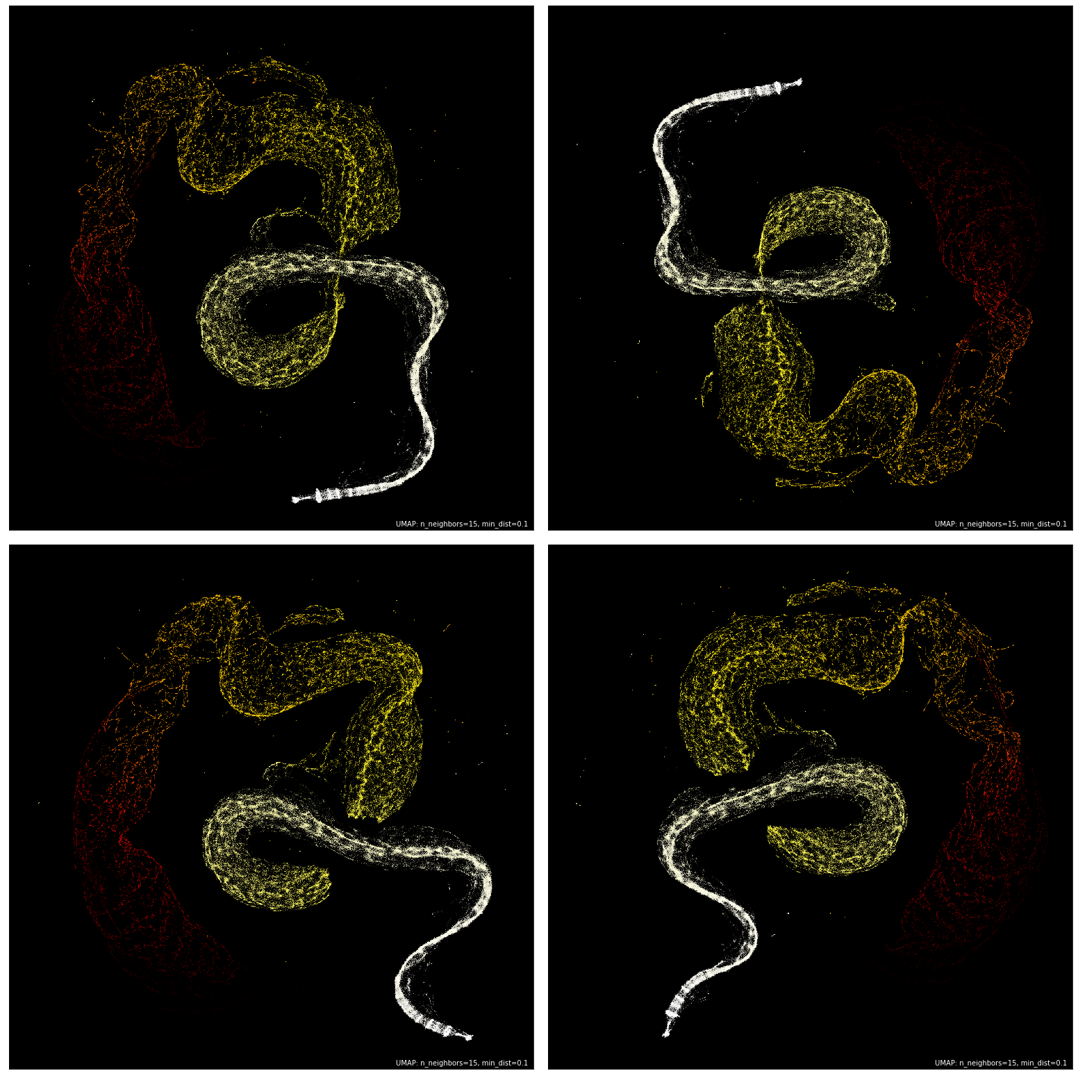
Another augmentation that could help refine this metric is examining the forward differences of each complexity curve instead of the raw data itself. I actually tried this and got another promising embedding:

Ultimately, I chose to spend the most time studying the embedding of the raw data because I did not want to impose my own nuanced constructions on the data. There is certainly much more that could be done to pre-process this data before embedding, and I am excited for what results that may yield.

Reproducibility

An important consideration is that UMAP is a non-deterministic algorithm. That is to say that each run of UMAP will most likely produce slightly different embeddings. I can verify that after running it around 50 times, the structure remained the same, but the orientation would sometimes differ.

Source Code and Data Explorer

I used various languages to generate and analyze this data. The automata simulator was written in C++, and the program to assemble histories of the complexity snapshots was written in Bash. PNG compression was done with Imagemagick via conversion from ASCII PPM (the simple output of the C++ simulation) to PNG. The Bash script saves the complexity histories as separate rows (one per each run) in a CSV file (one for each rule).

Then for the data analysis, I used Python to read in all of the CSV data and save it as a Numpy ndarray, while also averaging each of the ten trials I had generated for each of the rules. For each of the types of analysis I wanted to do, I made a Jupyter notebook that had access to Python 3 with all of the necessary dependencies for UMAP and displaying the results of the embeddings. The GitHub repo does not have the full data committed to the repository as the Gun-zipped tar-ball is just over half a gigabyte in size.

Lastly, I wanted a more natural way to explore the results and verify the structure of the embedding. I created a web-app using React and TerraJS that lets you select points in the serpent nebula and see what sort of automaton results from that point in the embedding. There is a zoomed view that shows neighboring points within a certain radius of the one that has been chosen. I also added the ability to enter rules and see where they are located in the serpent.

Here is a live demo of the app. Both the view of the full nebula and the zoomed portion are clickable, it just takes a second to find the closest rule. Please note that the page will take a few seconds to load as initializing the data for all quarter million rules is a processor-heavy task. As a result, I don’t expect mobile performance to hold up (or even work). I’m open to PR’s to improve the app.