Crouching Trig, Hidden Fractal

In some esoteric need to further my math addiction, I recently purchased a HP48 Reverse Polish Notation calculator. I was demonstrating the workings of the stack to my friend, and how each trig function supported complex numbers out-of-the-box. I absentmindedly entered \(4 + 5i\) into the stack, then pressed each trig key in sequence: \(\sin\), \(\cos\), \(\tan\). I was really surprised to see that the result was not some unwieldy floating point, but rather was simply:

\[ \tan(\cos(\sin(4+5i))) = i \]

To understand why this was surprising, it is important to note that sin, cos, and tan are all transcendental functions. This means that you cannot express any of these functions using a polynomial with a finite amount of terms. Also, these functions are periodic with respect to multiples of pi, which itself is irrational and transcendental. For real numbers, at least, these functions never have integer output for integer input (unless zero). More formally, you cannot form a set of integers that is closed under any of these functions.

Gaussian Integers resemble the integers in a few ways, but in general are a different beast. They are defined as any complex number \(a+bi\) such that \(a\) and \(b\) are integers.

Since there is no total ordering in a two-dimensional space, many properties found in the real integers do not apply. Primality, for example, is something much more difficult to define and intuitively grasp. Multiplication in the world of complex numbers is rotation and scaling, which we have a bad intuition over whenever composing operations.

For whatever reason though, it seems that a Gaussian Integer input to this composition of trig functions mapped to a Gaussian integer on output. There is a good chance that the number is not exactly a Gaussian Integer, but floating point error and numerical approximation makes it so. These functions are represented by Taylor Series in the processor, which are never exact representations of the true transcendental function.

\[ \cos(x) = \displaystyle \sum_{n=0}^\infty \frac{x^{2n}(-1)^{2n}}{2n!} \approx 1 - \frac{x^2}{2} + \frac{x^4}{24} + \mathcal{O}(x^6) \]

It seems to be accurate within many decimal places though, even when using orders of approximation far lower than what the calculator must use:

\[ cos(1) = 0.540302\dots \] \[ cos(1) \approx 1 - \frac{1}{2} + \frac{1}{24} = 0.541666 \]

In any case, I wanted to see what other Gaussian Integers mapped to Gaussian Integers under the function I was testing. I fired up Python and hacked together a few tests. First, I needed a way of getting my hands on some samples.

# @param {width} - Width of spatial domain
# @param {samples} - sample count along one side
# @return - square grid of samples at even intervals
def grid_sample(width, samples):
    out = []
    radius = int(round(samples/2))
    ds = width / float(samples)

    for a in range(-radius, radius + 1):
        for b in range(-radius, radius + 1):
            out.append(a*ds + b*1j*ds)

    return out

print grid_sample(3, 3)

Resulting in a 3x3 sample:

[(-1-1j), (-1+0j), (-1+1j), -1j, 0j, 1j, (1-1j), (1+0j), (1+1j)]

I then filtered the samples to see if there were any more oddities like the case I found.

from cmath import sin, cos, tan

def is_gaussian_integer(z, epsilon = 1e-20):
    return (
        abs(z.real - round(z.real)) < epsilon and
        abs(z.imag - round(z.imag)) < epsilon
    )

def predicate(z):
    try:
        result = tan(cos(sin(z)))

        return is_gaussian_integer(result)
    except:
        # If the result is infinite, we end up here
        return False

cases = filter(predicate, grid_sample(100, 100))

print "There are {} cases.".format(len(cases))

There are 1008 cases.

There was hundreds! Now I wondered what that might look like in the Complex Plane. I used Python Image Library to render a quick image where inputs that mapped to Gaussian Integers would be colored blue, and otherwise be left black.

# In pixels
imageWidth, imageHeight = 100, 30
image = Img.new("RGB", (imageWidth, imageHeight))

# In pixels per spatial unit
granularity = 1

# Find the location of a complex number in the image
# @param dim - in spatial units
# @param offset - in pixels
# @return - in pixels
def to_image_coord(dim, offset):
    return int(round(dim*granularity + offset/2))

# Color a pixel for each case we found
for sample in cases:
    x = to_image_coord(sample.real, imageWidth)
    y = to_image_coord(sample.imag, imageHeight)
    coord = (x, y)

    if 0 <= x < imageWidth and 0 <= y < imageHeight:
        image.putpixel(coord, (0, 0, 255))

image.show()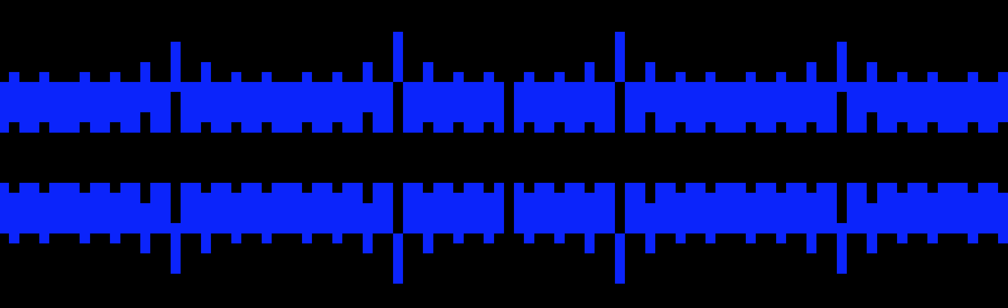

This was more surprising. The numbers seemed to exhibit some periodicity, but also symmetry about the real axis. I abandoned my search for closure over some subset of Gaussian Integers for a moment and wanted to look deeper into this pattern. I began to test for non-integer inputs with the same property, and also re-wrote the algorithm a bit so that it only tested a sample per output pixel.

transform = lambda z: tan(cos(sin(z)))

# In pixels
imageWidth, imageHeight = 500, 340
image = Img.new("RGB", (imageWidth, imageHeight))

# In pixels per spatial unit
granularity = 10

for u in range(imageWidth):
    for v in range(imageHeight):
        real_part = (u - imageWidth*0.5)/granularity
        imag_part = (v - imageHeight*0.5)/granularity

        try:
            # This could be "infinite", thus the try/except
            result = transform(real_part + imag_part*1j)

            if is_gaussian_integer(result, 1e-100):
                image.putpixel((u, v), (0, 0, 255))
        except:
            pass

image.show()

This was the result:

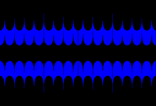
I feel like I’ve seen this fractal before. I recognize that different functions would produce different fractals, but the complexity in this answer really surprised me. Even when trying different functions, I still got fractal results:

Curious to see if this was a product of floating point error, I started coloring the domain based upon just how close the output got to a Gaussian Integer.

# Color Scheme
colors = [
    (239, 71, 111),
    (255, 209, 102),
    (17, 138, 178),
    (6, 214, 160),
    (7, 59, 76),
]

transform = lambda z: tan(cos(sin(z)))

# In pixels
imageWidth, imageHeight = 1440, 900
image = Img.new("RGB", (imageWidth, imageHeight))

# In pixels per spatial unit
granularity = 30

for u in range(imageWidth):
    for v in range(imageHeight):
        real_part = (u - imageWidth/2.0)/granularity
        imag_part = (v - imageHeight/2.0)/granularity

        try:
            # This could be "infinite", thus the try/except
            result = transform(real_part + imag_part*1j)

            if is_gaussian_integer(result, 0):
                image.putpixel((u, v), colors[4])
            elif is_gaussian_integer(result, 1e-100):
                image.putpixel((u, v), colors[3])
            elif is_gaussian_integer(result, 1e-10):
                image.putpixel((u, v), colors[2])
            elif is_gaussian_integer(result, 1e-1):
                image.putpixel((u, v), colors[1])
        except:
            image.putpixel((u, v), colors[0])

image.show()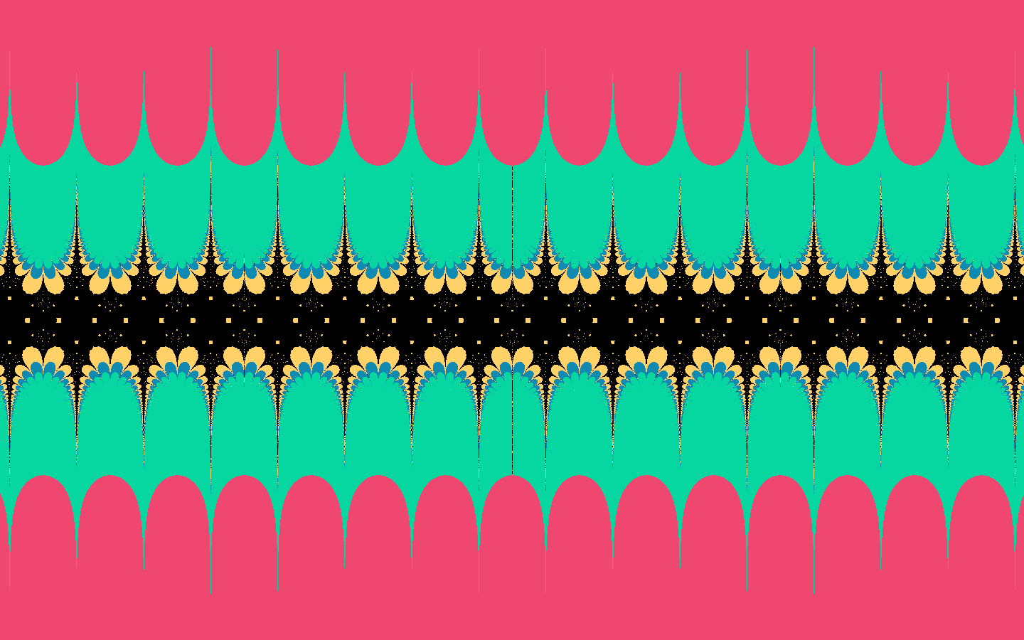

I think this one turned out the coolest. The yellow pixels represent inputs that (according to Python’s test of equality and the limitations of floating point representation) map exactly to Gaussian Integers. Here is a closer look at the internal region where it looks like the set becomes disconnected:

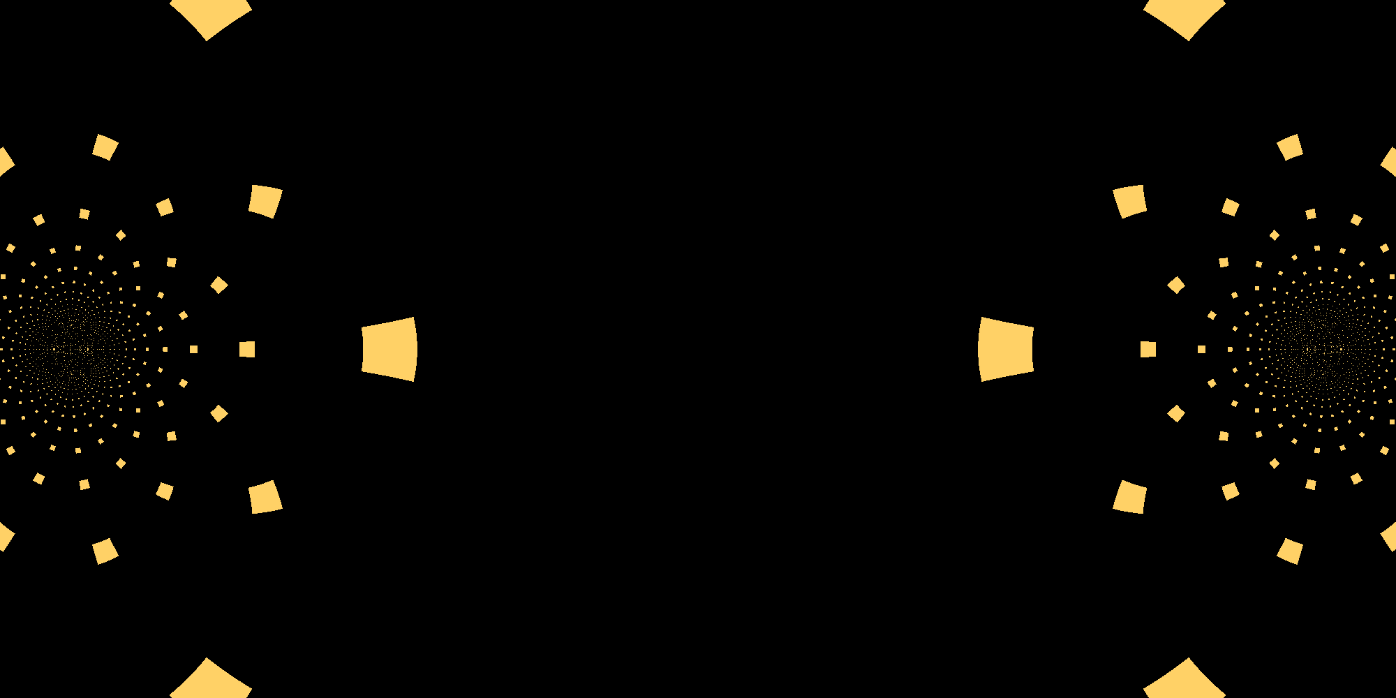
(Note that this is rotated 90 degrees to fit on the page better). Why are there squares, apparently conformally mapped about poles? I think that these represent points that map to Gaussian Integers under the function I am examining, and the width/height of the squares is the smallest number my computer can represent in this context.

Closing Thoughts

I end this exploration with no real conclusion as to why these fractal regions of the complex plane map to Gaussian Integers under these functions. Is this fact extant without numerical approximation? I still have many unanswered questions about these fractals, and hope to one day get to the bottom of this.